Constrain, load, and solve · M00 · Learn to Program Ansys APDL Simulations

Complete the PREP7 → SOLU → POST1 flow while tracking which entities are selected.

Block 4 — Select and constrain

NSEL,S,LOC,X,0
D,ALL,ALL,0
ALLSEL,ALL

NSEL,S,LOC,X,0 replaces the current selection with the nodes located in x=0. D,ALL,ALL,0 restricts all of its available degrees of freedom. Finally, ALLSEL,ALL retrieves all entities.

Selection is status

Many commands act only on the selected one. Forget ALLSEL can make stages ignoring much of the model without the problematic line appearing incorrect.

Block 5 — Distribute the total force

NSEL,S,LOC,X,1.0
*GET,n_tip,NODE,0,COUNT
F,ALL,FY,-1000/n_tip
ALLSEL,ALL

The end nodes are selected first. *GET count how many there are and save the result en n_tip. The strength of each node is -1000/n_tip, so the sum remains equal to − 1000N even if you change the mesh.

This idea is important: the input value represents a total force, not a force that must be repeated in full at each node.

Block 6 — Exit PREP7 and Solve

FINISH

/SOLU
ANTYPE,STATIC
SOLVE
FINISH

FINISH exits the current processor and returns to BEGIN.
/SOLU goes into Solution.
ANTYPE,STATIC declares a static analysis.
SOLVE requests the solution of the current load step.
The second FINISH closes the solution stage.

That SOLVE finish only proves that the solver got an answer. We still have to check if it correctly represents the physical problem.

Block 7 — Enter POST1

/POST1
SET,LAST
PLNSOL,U,SUM
PLNSOL,S,EQV
FINISH

/OUTPUT

/POST1 opens the general postprocessor.
SET,LAST read the latest set of results available.
PLNSOL,U,SUM represents the magnitude of the displacement.
PLNSOL,S,EQV represents the equivalent stress.
/OUTPUT with no arguments returns live text output to the Output Window.

Each plot replaces the previous one in the viewport. At the end you will see the equivalent stress. You can rerun PLNSOL,U,SUM manually to restore the displacement contour.

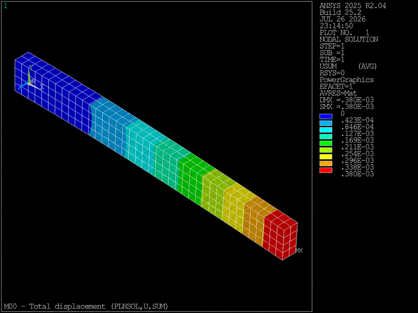
MAPDL contour of total displacement PLNSOL U SUM after the first SOLVE — Figure 5. Total displacement contour (`PLNSOL,U,SUM`). It connects the model to its results; it does not demonstrate convergence or analytical validation.

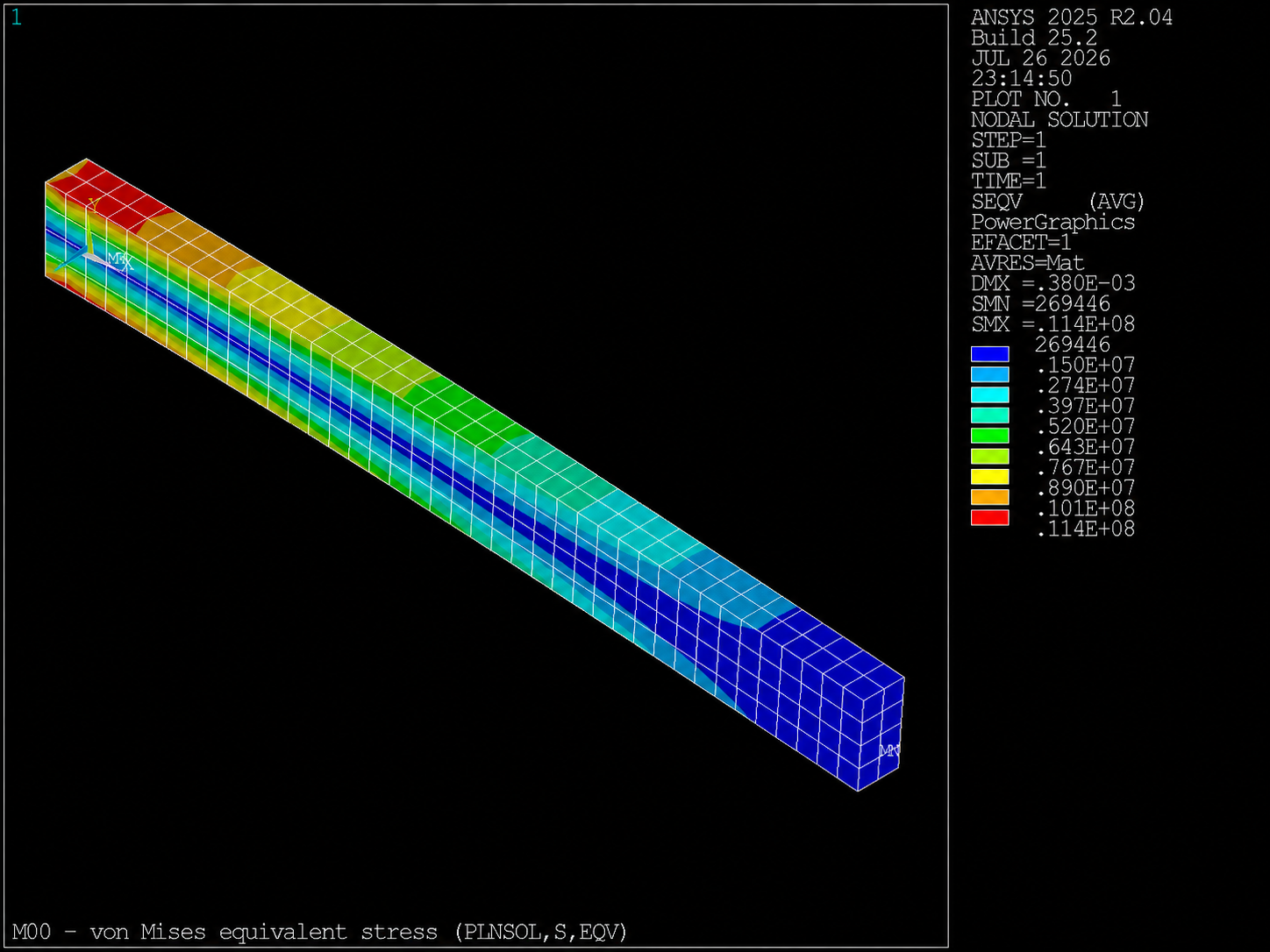
Von Mises PLNSOL S EQV equivalent stress MAPDL contour — Figure 6. Von Mises equivalent stress (`PLNSOL,S,EQV`). A second type of visual inspection; it does not replace the linearity challenge tolerances.