
In M06 we showed that the beam was in equilibrium. That still does not answer the more important question: Does it correctly represent the structure we intended to study? In M07 we will turn contour plots into comparable quantities and defensible decisions.
Your mission
You will measure the average deflection of the tip face, extract the normal stress at an interior section, and compare both quantities with beam theory. The resulting CSV will record whether the model passes or fails the validation criteria.
Guiding question: Does a visually reasonable contour constitute validation?
Objectives
By completing M07 you will be able to:
- Distinguish visualization, extraction and validation.
- Deliberately select the result set and coordinate system.
- Extract results using
*GETwithout depending on IDs. - Represent a section using an average and a spread.
- Compare the FEA deflection with Euler–Bernoulli.
- Compare
S,Xwith normal bending stress. - Distinguish averaged and non-averaged results.
- Prevent a singularity from governing a global conclusion.
Prerequisites and downloads
- M04: The 40-element mesh is converged for tip displacement.
- M06: a set exists and the balance of forces and moments is closed.
- M01: the analytical expressions for deflection and nominal stress are available.
07_start.mac— starting point.07_post_validation.mac— audited solution.07_bug_hunt.mac— five misleading validation approaches.07_challenge.mac— scaling challenge.07_expected_results.csv— self-checking contract.07_graphics_post26.mac— extension: PNG output and a load–response curve.07_graphics_challenge.mac— constant slope challenge.07_graphics_expected_results.csv— expansion contract.validation-ladder.svg— trust ladder.stress-probe-vs-singularity.svg— stress section.
How to use this lesson
| Track | Duration | Scope |
|---|---|---|
| Quick win | 35–40 min | Prediction, deformation inspection and mean deflection extraction. |
| Complete | 70–75 min | Additionally, interior stress validation, balance, scaling challenge and CSV. |
| Graphic expansion (optional) | 25–30 min | Reproducible PNG plots, the m07_load_response.csv table, and a first curve with /POST26. |
Keep visualization, extraction, and validation separate. A plausible contour plot is no substitute for comparison with an analytical reference and a justified tolerance.
Session map
- Mission: goals, downloads and analytical prediction.
- Mental model: trust ladder, not a single verdict.
- Demo: deflection, interior stress, and preserved equilibrium.
- Bug hunting: singularities and wrong magnitudes.
- Challenge: double the length with verifiable reasons.
- Extension (optional): Reproducible graphs and load–response curve with POST26.
- Mastery: final test that records demonstrated mastery and recommends M08.
Prediction — Simulation starts before the solver
For the rectangular section:
I = b·h³/12
I = 0.05·0.10³/12 = 4.16667E−6 m⁴
The Euler–Bernoulli tip deflection at the end is:
uy_ref = F·L³/(3·E·I)
uy_ref = −3.80952E−4 m = −0.380952 mm
M07 uses KEYOPT(2)=3 and obtains approximately
−3.79470E−4 m at the corner node. Before running
M07, we can already predict an average deflection error on the order of
1 %, less than the limit of 5 %.
Mental model — A ladder, not a verdict
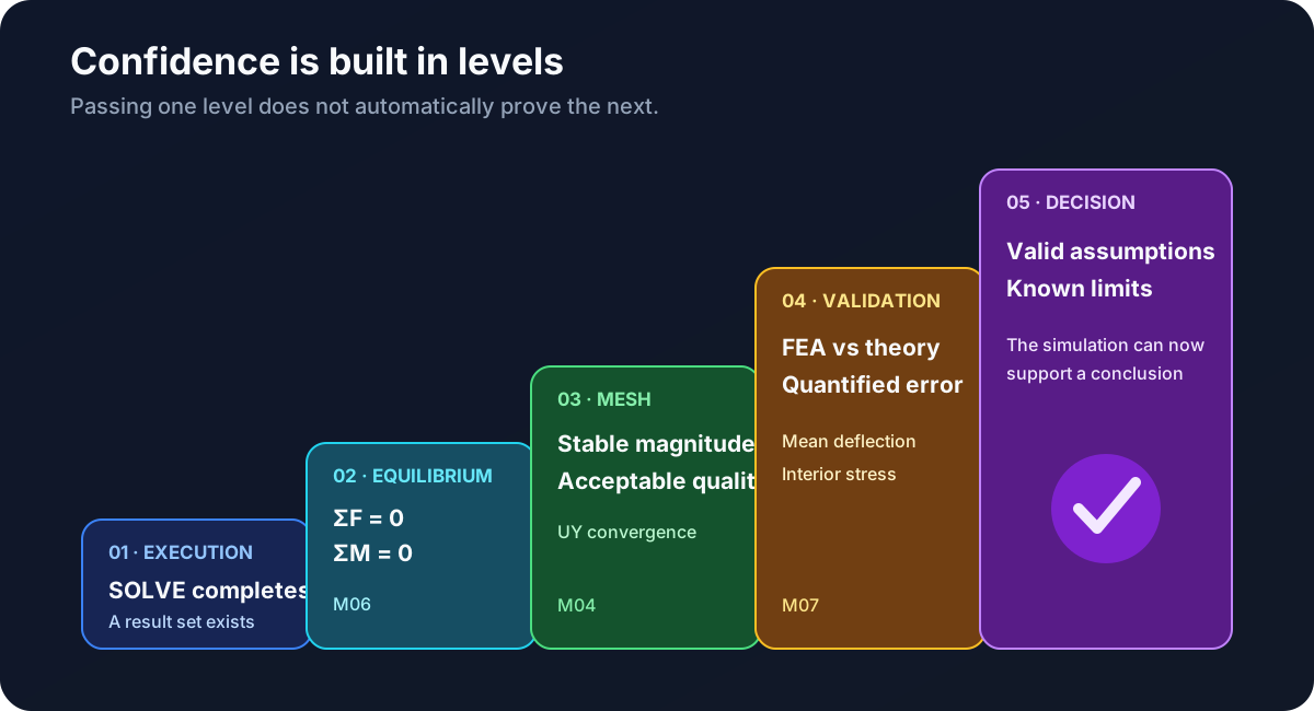
A completed solution may still violate equilibrium. A balanced model may remain mesh-dependent. A converged quantity may still rest on incorrect physical assumptions. M07 does not replace the previous checks; it incorporates them as preconditions.
Three verbs that do not mean the same
- View
- Recognize deformed shape, critical areas, signs and discontinuities.
- Extract
- Convert a specific result into a reproducible parameter.
- Validate
- Compare that parameter with independent evidence and a justified tolerance.
PLNSOL helps you interpret the result, but it does not generate quantitative evidence by itself.
*GET extracts a number, but does not validate it either. Validation requires a defined
reference, error measure, and decision rule.
Activate the correct state
/POST1
*GET,n_sets,ACTIVE,0,SET,NSET

*IF,n_sets,GE,1,THEN
  SET,LAST
  solution_available=1
*ENDIF

RSYS,0
SET,LAST loads the last stored result set. RSYS,0 expresses the
results in global Cartesian coordinates. This matters especially for
S,X: a component without a declared coordinate system is incompletely defined.
First inspection — The deformed shape
/GRAPHICS,POWER
PLDISP,2
Before looking at stresses, check that the deformation corresponds to the expected mechanism: zero displacement at the support, downward tip motion, and smooth curvature. An unexpected shape should be investigated before calculating error percentages.
The plot scale factor may exaggerate the deformation. Use the scaled shape to recognize the pattern, not to measure the deflection visually.
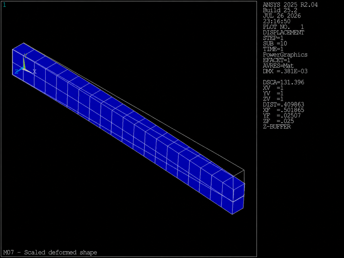
PLDISP,2). The exaggerated scale reveals the mechanism; it does not show the true displacement magnitude.
Why a node does not necessarily represent a section
M04 needed an identical probe between meshes and used the geometric node
(L,0,0). M07 asks a slightly different question: how far does the
entire end section move?
To answer we will use all the nodes of tip_nodes and we will keep the
M04 node as secondary control. This way we avoid turning a particular corner into a
property of the entire face.
Extract the average deflection
CMSEL,S,tip_nodes
node_id=0
uy_sum=0

*DO,j,1,n_tip
  node_id=NDNEXT(node_id)
  *GET,uy_node,NODE,node_id,U,Y
  uy_sum=uy_sum+uy_node
*ENDDO

uy_tip_avg=uy_sum/n_tip
The pattern is familiar: select → scan → read → accumulate. The difference is that
*GET now reads the result set rather than the geometry or loads.
Average and dispersion tell different stories
In addition to the average we keep:
uy_tip_min
uy_tip_max
uy_spread = uy_tip_max−uy_tip_min
uy_spread_ratio = |uy_spread|/|uy_tip_avg|
The average approximates the translation of the section. The spread indicates whether the face moves
almost like a rigid section or presents significant warping and local variations. M07
requires a dispersion less than 1 %.
Traceability with M04
NSEL,S,LOC,X,beam_l
NSEL,R,LOC,Y,0
NSEL,R,LOC,Z,0
*GET,corner_node,NODE,0,NUM,MIN
*GET,uy_tip_corner,NODE,corner_node,U,Y
The ID is discovered only after the physical location is defined. With
KEYOPT(2)=3, the value should reproduce
−3.79470E−4 m within 0.1 %. If it does not, M07 is not
analyzing the same validation model.
The reference is not the absolute truth
Euler–Bernoulli assumes, among other things:
- linear, homogeneous and isotropic material;
- small deformations;
- flat sections that stay flat;
- negligible shear deformation;
- idealized load and support.
The 3D solid is not identical to that one-dimensional model. A small error supports consistency between them, but even a perfect match would not prove that every assumption is correct.
Displacement error
inertia=beam_b*beam_h**3/12
uy_ref=tip_force*beam_l**3/(3*young*inertia)
uy_error=ABS(uy_tip_avg-uy_ref)/ABS(uy_ref)
The comparison retains the sign in the original values and uses magnitudes only
in the denominator of the error. Acceptance requires uy_error<0.05.
Which stress should we compare?
Beam theory predicts longitudinal normal stress. Therefore, compare it with
S,X, not with von Mises stress:
sigma_x = M(x)·y/I
S,EQV combines components using an energy criterion and is useful for other
decisions, but it does not represent the same magnitude as the previous equation.
Do not use the fixed support to characterize the beam
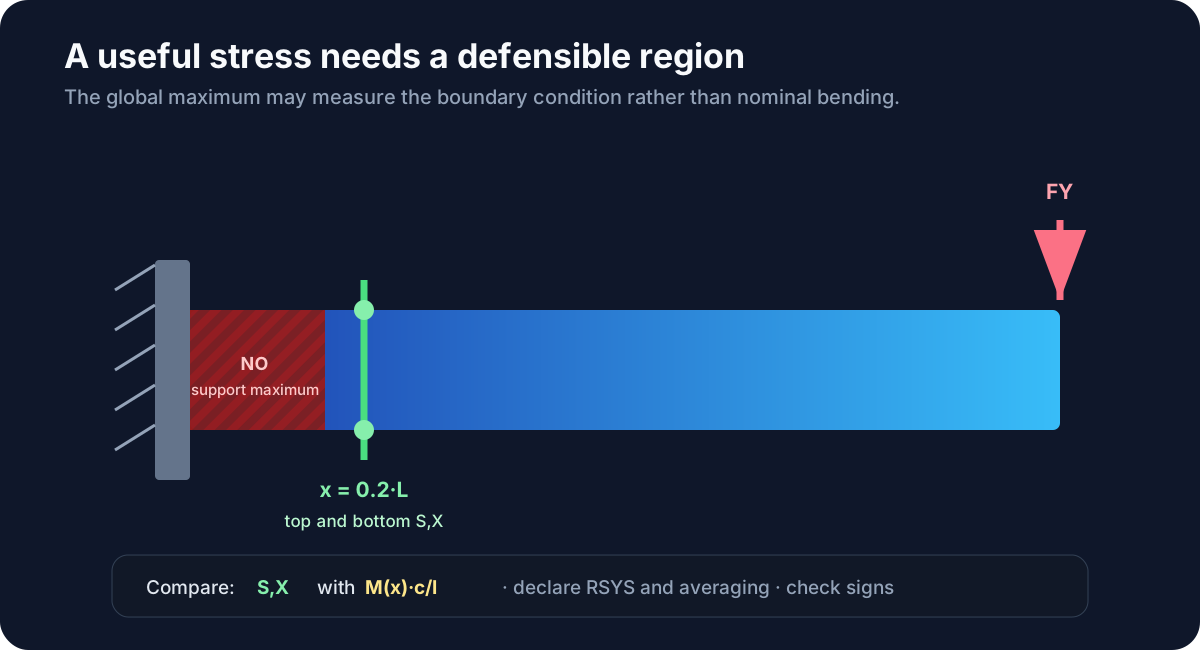
x=0.2·L.
At the fixed support, zero displacement is imposed on an entire face. The transition from that idealization to the deformable field creates mesh-sensitive stress concentrations. Using the maximum stress as the sole validation metric mixes nominal behavior with a local disturbance.
Stress reference in the interior section
x_section=0.2*beam_l
moment_section=ABS(tip_force)*(beam_l-x_section)
sigma_ref=moment_section*(beam_h/2)/inertia
For the base case:
M(0.2L) = 1000·(1−0.2) = 800 N·m
sigma_ref = 9.6 MPa
The section is two element lengths from the fixed support and sufficiently far from the load application.
Extract the upper and lower fibers
NSEL,S,LOC,X,x_section
NSEL,R,LOC,Y,beam_h
CM,stress_top_nodes,NODE

*GET,sx_node,NODE,node_id,S,X
The base mesh contains two nodes across the width at the top fiber and two at the
bottom fiber. We average each pair separately. For a force in the −Y direction,
we expect:
sx_top_avg > 0     ! tension
sx_bottom_avg < 0  ! compression
Magnitude and antisymmetry
sigma_fea=(ABS(sx_top_avg)+ABS(sx_bottom_avg))/2
stress_error=ABS(sigma_fea-sigma_ref)/sigma_ref
stress_symmetry=ABS(ABS(sx_top_avg)-ABS(sx_bottom_avg))/sigma_ref
The first metric checks the nominal magnitude. The second verifies that the extreme fibers
develop opposite stresses of similar magnitude, as predicted by pure bending.
Their respective limits are 10 % and 5 %.
PLNSOL vs. PLESOL
PLNSOL,S,X
PLESOL,S,XPLNSOLrepresents nodal values averaged across compatible elements.PLESOLpreserves the values of each element and leaves the breaks visible.
A smoother contour is not automatically more precise. Comparing both views helps detect how much the averaging is hiding.
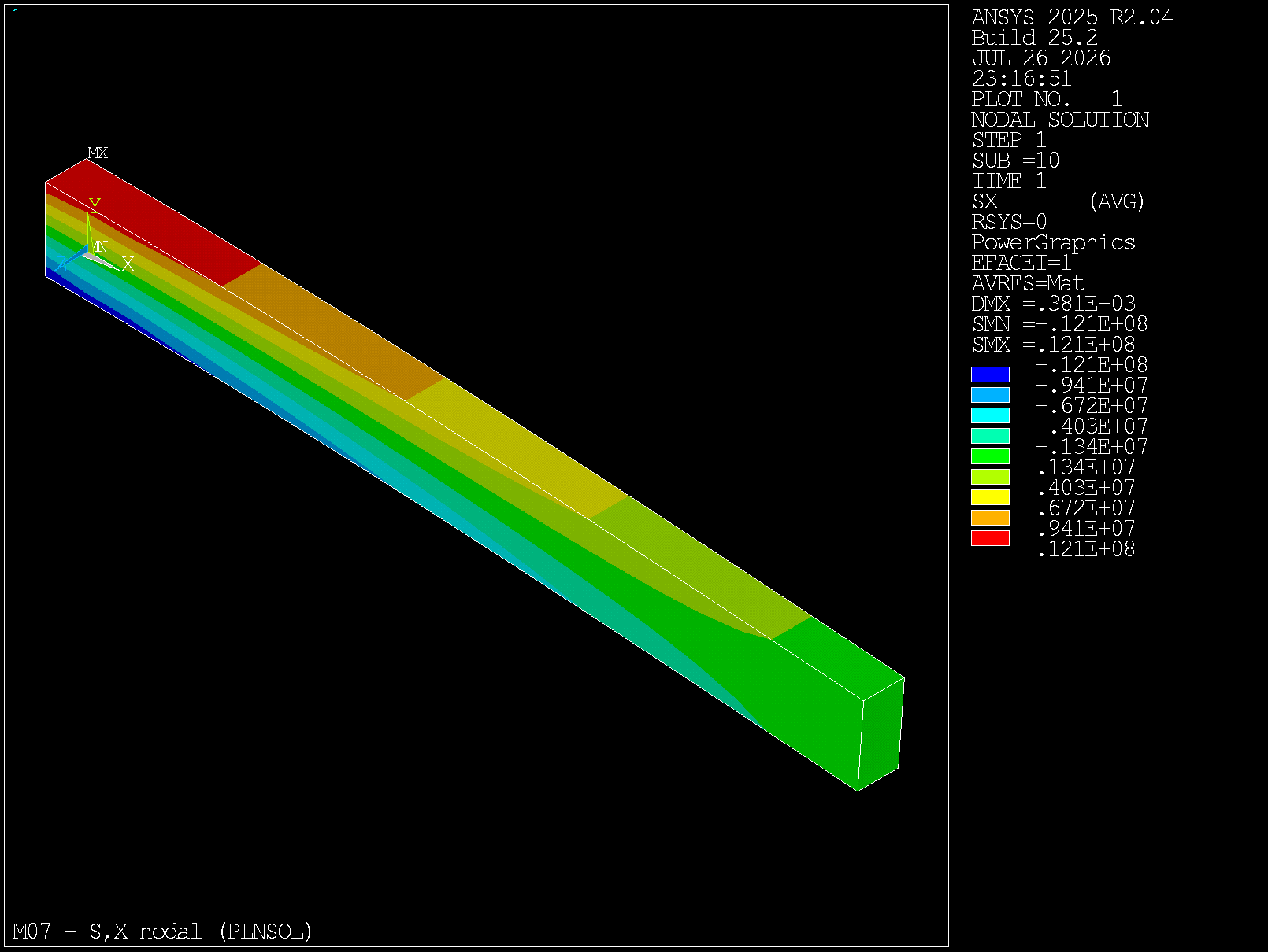
S,X stress (PLNSOL,S,X) in the interior section.
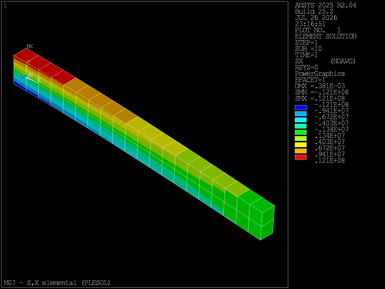
S,X stress (PLESOL,S,X). The key contrast with PLNSOL is that jumps remain visible at interfaces.
Reproducible graphics with POST1
On-screen contours are useful for inspection, but a manual screenshot is not reproducible
evidence. Before plotting, activate the correct set with SET,LAST and declare
RSYS,0. Then redirect the graphical output with /SHOW,PNG
(not /SHOW,nombre,PNG, which writes invalid ANSYS raster as PNG):
/GFILE,1200
/DEVICE,VECTOR,1
/GRAPHICS,POWER
/SHOW,PNG
/TITLE,M07 - UY nodal (PLNSOL)
/AXLAB,X,X (m)
/AXLAB,Y,Y (m)
PLNSOL,U,Y
/SHOW,CLOSE
/GFILE sets the resolution; /TITLE and /AXLAB document
what the plot represents; /SHOW,CLOSE closes the graphics device. MAPDL writes
Jobname000.png, Jobname001.png, etc.; rename them if you need
descriptive names. Repeat the workflow for
PLDISP, PLNSOL,S,X and PLESOL,S,X.
Interpret the scale carefully: the deformation factor of PLDISP exaggerates the
shape; the contour legend can hide jumps between nodes and elements; units must
match /UNITS,SI. A well-labeled PNG helps communicate the result, but it does not
replace the validation CSV.
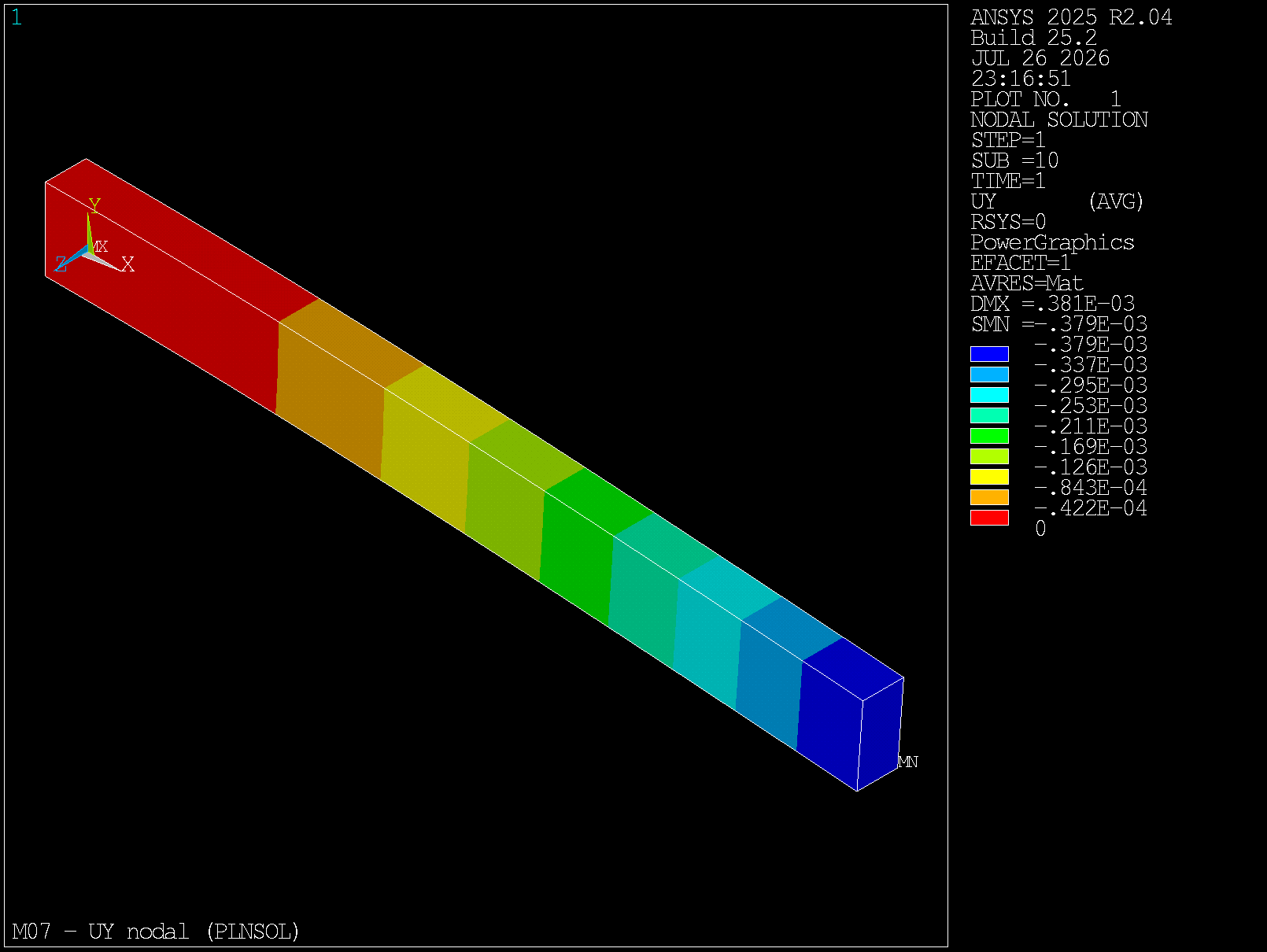
UY (PLNSOL,U,Y).
Validation preserves balance
M07 audits reactions and moments again. If a postprocessing change requires us to rebuild or solve the model, we must show that the M06 prerequisite remains satisfied:
force_error  < 0.005
moment_error < 0.005
Validation does not replace equilibrium; it depends on it.
Acceptance contract
The case receives passes=1 only when all of the following conditions are met:
- 126 nodes, 40 elements, 6 tip nodes, and at least one result set.
- Deflection error less than
5 %. - Tip-face displacement spread below
1 %. - Corner node consistent with M04 within the
0.1 %. - Two top and two bottom nodes in the section.
- Correct tension and compression signs.
- Stress error less than
10 %. - Stress asymmetry less than
5 %. - Balance errors less than
0.5 %.
CSV — A complete record of the comparison
The macro generates m07_validation_audit.csv:
case,beam_l,mesh_h,n_nodes,n_elements,n_sets,n_tip,
uy_tip_avg,uy_tip_corner,uy_tip_min,uy_tip_max,uy_spread,
uy_ref,uy_error,x_section,n_top_section,n_bottom_section,
sx_top_avg,sx_bottom_avg,sigma_fea,sigma_ref,
stress_error,stress_symmetry,force_error,moment_error,passes
The CSV preserves model, measurement, reference, error and decision. This allows repeating the validation without reconstructing the interpretation from screenshots.
Guided practice
- Calculate manually
I,uy_refandsigma_ref. - Run the model until
SOLVEand confirm the set. - Inspect the deformation before extracting results.
- Calculate the average and dispersion of
tip_nodes. - Reproduce the M04 corner probe geometrically.
- Extract
S,Xtop and bottom in0.2·L. - Compare
PLNSOLandPLESOL. - Generate the CSV and justify each tolerance.
Bug hunting — Five convincing results
- Implicit set: results are queried without knowing which set is active.
- Fixed ID: numerical identity is confused with physical location.
- Different magnitudes: von Mises is compared with normal stress.
- Singular maximum: the fixed-support stress governs the entire conclusion.
- Hidden transformation: neither
RSYSnor the averaging method is declared.
For each case, identify the number that might seem reasonable, the physical question that number actually answers, and the evidence that is missing.
Challenge — Double the length
Keep the cross-section, material, force and mesh_h=0.05 m, but use:
beam_l=2.0The new topology will have 80 elements and 246 nodes. The theory predicts:
uy_ref_2 = −3.04762E−3 m
uy_2/uy_1 = 8

x_section_2 = 0.4 m
sigma_ref_2 = 19.2 MPa
sigma_2/sigma_1 = 2
Both FEA ratios should approach the predictions within the 5 %, and the
both cases must continue to satisfy equilibrium.
Optional expansion — POST1 vs. POST26
This extension is not part of the M07 approval contract. It serves to distinguish two different questions:
/POST1- Represents a spatial field in a specific set: deformed shapes, contours, and point listings.
/POST26- Tracks a quantity across multiple sets: load–response curves or time histories.
The script 07_graphics_post26.mac solves the same case with a static ramp
(KBC,0), NSUBST,10 and OUTRES,ALL,ALL. In this context
TIME acts as a normalized load factor, not as physical
time. M14 will revisit /POST26 with an actual time history.
Load–response curve with POST26
/POST26
NUMVAR,10
NSOL,2,corner_node,U,Y
XVAR,1
/AXLAB,X,Load factor (TIME)
/AXLAB,Y,UY at corner node (m)
/SHOW,PNG
PLVAR,2
/SHOW,CLOSE
PRVAR,1,2
NSOL defines the variable, PLVAR draws the curve, and PRVAR
lists the points. To ensure that the graph is not the only evidence, the script also generates
m07_load_response.csv walking through the sets in POST1:
substep,load_factor,uy_corner_m,uy_ratio_to_final
Prediction: at 50 % load, UY should be approximately
half of the final value in a linear analysis. The expansion contract requires an error of
intermediate linearity lower than 2 %.
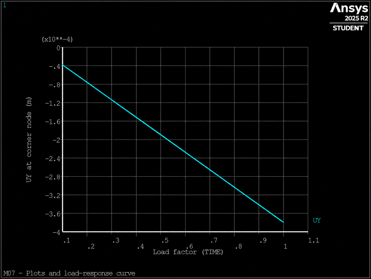
POST26, PLVAR,2). Intermediate linearity verified in m07_load_response.csv.
Extension challenge — Constant slope
Run 07_graphics_challenge.mac with final loads of
−500 N and −1000 N. Check that the slope
UY/F remains constant within the 2 %. The file
m07_graphics_slope_audit.csv documents both cases.
Self-assessment
- What is the difference between visualizing and validating?
- Why is average deflection the primary metric?
- What does preserving the M04 node provide?
- Why is it fixed
RSYS,0? - Why should
S,EQVnot be compared withM·c/I? - What difference exists between
PLNSOLandPLESOL? - What question does POST1 answer and what question does POST26 answer?
- What would it mean if the deflection converges but the interior stress does not?
See short answers
- Visualization shows patterns; validation compares a quantity with independent evidence.
- Because it represents the translation of the entire section and reduces dependence on a corner.
- It shows that we continue solving the same case used in convergence.
- To declare the system in which we interpret the components.
- Because von Mises and longitudinal normal stress are different magnitudes.
- The first averages nodally; the second shows values element by element.
- POST1 displays a field in a set; POST26 shows a magnitude across sets.
- That a mesh accepted for displacement is not necessarily validated for stress.
Evidence of learning
m07_validation_audit.csvwith entries, references and errors.- Manual deflection and stress predictions.
- Comparison between face mean and corner node.
PLNSOLandPLESOLcontour plots ofS,X.- Diagnosis of the five misleading validation approaches.
m07_scaling_audit.csvwith the reasons for the challenge.- POST26 contour and curve PNG generated by
07_graphics_post26.mac. m07_load_response.csvandm07_graphics_slope_audit.csv(expansion).
Exit checklist
- ☐ I identify and activate the set I analyze.
- ☐ I declare the results system.
- ☐ I inspect the deformed shape before examining stress.
- ☐ My probe represents a physical region, not an ID.
- ☐ I compare equivalent magnitudes.
- ☐ I avoid using the singular fixed-support maximum.
- ☐ I document the averaging method, reference, and tolerance.
- ☐ I maintain balance and traceability with previous modules.
- ☐ (Optional) I distinguish POST1 from POST26 and export graphics with metadata.
Technical traceability
The lesson uses Structural Analysis Guide for post processing,
Theory Reference for the interpretation of results,
Element Reference for the outputs of SOLID185 and
Command Reference 2024 R1 for /POST1, /POST26, SET,
RSYS, /SHOW, /GFILE, /TITLE, /AXLAB,
PLDISP, PLNSOL, PLESOL, PLVAR, PRVAR,
NSOL, NUMVAR, PRNSOL, NDNEXT and *GET.
Next step: M08
We already have a model that is built, solved and validated. In M08 we will convert it into a reusable tool using macros, arguments, files and a strategy of systematic debugging.